
Hello guys, welcome to this new project of Generating Fake Faces. There is a wonderful concept called GANs (Generative Adversarial Network) which generates fake images. You can generate any thing you want. If you have person's faces dataset, you can generate fake faces of persons. If you have Pokémon's dataset, you can generate new Pokémon that never exists on the Earth. GANs were invented by Ian Goodfellow in 2014 and first described in paper Generative Adversarial Nets. If you have zero knowledge about GANs don't worry about it, you will learn how it works here and by the end of the post you will be able to generate whatever you want (only if you have a good and huge dataset!!!). One last thing I want to inform you is that this project is done using PyTorch. You can find the full code here. You can find more fake persons that doesn't exist on the earth here, once go through it. OK guys lets start our project.
 |
Generative Adversarial Networks
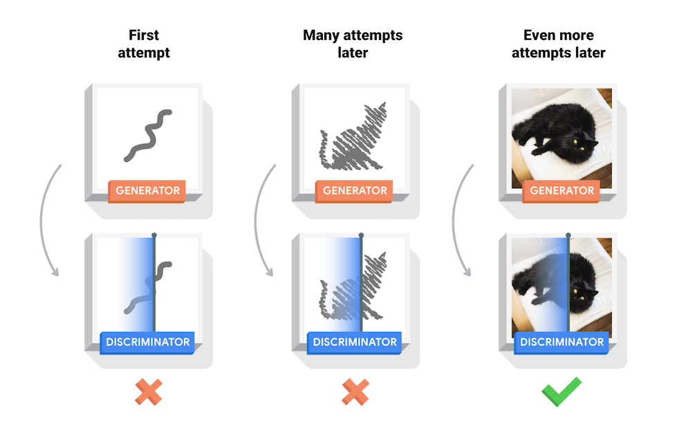
Generative Adversarial Networks (GANs) are one of the most interesting ideas in computer science today. Here two models named Generator and Discriminator are trained simultaneously. As the name says Generator generates the fake images or we can say it generates a random noise and the Discriminator job is to classify whether the image is fake or not. Here the only job of Generator is to fake the Discriminator. If you didn't understand anything, don't worry about it, we will be discussing two models (Generator and Discriminator) separately. Before that I want to talk little bit about Pytorch!
Pytorch
Pytorch was introduced by the Facebook AI Research (FAIR) team, back in early 2017, and has become a highly popular and widely used Deep Learning (DL) framework.
Tensors: Tensors are at the heart of any DL framework. PyTorch provides tremendous flexibility to a programmer about how to create, combine, and process tensors as they flow through a network (called computational graph) paired with a relatively high-level, object-oriented API
 |
- Scalar are 0-dimensional tensors.
- Vectors are 1-dimensional tensors.
- Matrices are 2-dimensional tensors
- Tensors are generalized N-dimensional tensors. N can be anything from 3 to infinity…
If you want to learn more about Pytorch please refer to the official website of Pytorch. Now let's talk about Generator and Discriminator in detail. In this project we are using DCGAN(Deep Convolutional Generative Adversarial Network). A DCGAN is a direct extension of the GAN described above, except that it explicitly uses convolutional and convolutional-transpose layers in the discriminator and generator, respectively. DCGANs actually comes under Unsupervised Learning and was first described by Radford et. al. in the paper Unsupervised Representation Learning With Deep Convolutional Generative Adversarial Networks.
Generator
 |
- First we have to provide a random noise to the generator as a input.
- Make sure that the Generator never ever sees the real images.
- The only job of generator is to generate fake images and to fool the discriminator. It gives the fake images to the discriminator and says "Hey, these are real Images!" to the discriminator.
- This is accomplished through a series of strided two dimensional convolutional transpose layers, each paired with a 2d batch norm layer and a relu activation.
- The output of the generator is fed through a tanh function to return it to the input data range of [-1,1].
Discriminator
 |
- For the discriminator there will be tow inputs, one from Generator(fake images) and the other is real images that should be given by us.
- It classifies whether the given image is of real face or not.
- Most probably for the first time the discriminator classifies all the images(random noise) from generator as fake images, because it is a random noise.
- The network looks quite opposite to the discriminator.
- As mentioned, the discriminator is a binary classification network that takes an image as input and outputs a scalar probability that the input image is real (as opposed to fake).
- Here, Discriminator takes a 3x64x64 input image, processes it through a series of Conv2d, BatchNorm2d, and LeakyReLU layers, and outputs the final probability through a Sigmoid activation function.
Loss function
Here,
- m is number of samples
- D(x) is Discriminator where x(i) is training examples
- G(z) is Generator where z(i) is latent vector or random noise
If you have idea about cost function, it is similar to it. Here we use Binary Cross Entropy as a loss function. Our aim is to make this loss function zero. To do that we want to make two terms zero(1st term = log(D(x(i))) and 2nd term is log(1 - D(G(z(i)))) )
Now let us consider 1st term,
To make 1st term zero we want to make D(x(i)) = 1. This means that the discriminator want to detect the training examples as real images. Most probably it is equal to 1. there is no problem with the 1st term.
Now let us consider 2nd term,
To make 2nd term zero we want to make D(G(z(i))) = 1. This means that when we pass the fake images generated from the Generator as input to the Discriminator, then Discriminator has to detect that fake images as real images. But how is it possible??
Before knowing the answer, we want to conclude that our loss value is the sum of loss values of two terms i.e., ''how bad the discriminator classifies the real images as real(1st term) and how bad the discriminator classifiers the fake images as real(2nd term).''
Ok, now let's come back to our question, How is it possible to make our 2nd term zero? Here comes the optimizers into the picture. Here we use Adam optimizer to reduce the loss function through back propagation. Finally, we set up two separate optimizers, one for Generator and one for Discriminator. As specified in the DCGAN paper, both are Adam optimizers with learning rate 0.0002 and Beta1 = 0.5.
By this way, we reduce our loss, fool the discriminator and generate the fake faces of persons.
Below figure shows how GANs work
 |
Now let's start coding!!!
Import necessary modules
import random
from  PIL import Image
import numpy as np
import matplotlib.pyplot as plt

import torch
import torch.nn as nn
import torchvision.datasets as datasets
import torchvision.transforms as transforms
import torchvision
I request every one not to train on CPU devices, because it take 24 hours to train the model. Please use Google Colab or any other which has GPU.
device = torch.device("cuda:0" if (torch.cuda.is_available()) else "cpu")
Download The Datasets
Here we used the Celba-A Faces dataset and you can download the dataset here. This is a zip file. You just download it and unzip the file. That's all!
Load the data
You can use the following code to load the data. PyTorch helps us a lot with its inbuilt modules. Here transform is used to compose the image, like converting to tensor, scaling the image and finally normalizing the image
img_size=64
batch_size=128
input_latent=100
transform = transforms.Compose(
[transforms.ToTensor(),
transforms.ToPILImage(),
transforms.Scale(size=(img_size, img_size), interpolation=Image.BICUBIC),
transforms.ToTensor(),
transforms.Normalize((0.5, 0.5, 0.5), (0.5, 0.5, 0.5))])
dataset = datasets.ImageFolder(root='./data_faces',transform=transform)
dataloader = torch.utils.data.DataLoader(dataset, batch_size=batch_size,shuffle=True)
Training Images
You can see some of the training images and how it looks like.
real_batch = next(iter(dataloader))
plt.figure(figsize=(8,8))
plt.axis("off")
plt.title("Training Images")
plt.imshow(np.transpose(torchvision.utils.make_grid(real_batch[0].to(device)[:64], padding=3, normalize=True).cpu(),(1,2,0)))
 |
Initialize weights
Don't be scared from the code below. From the DCGAN paper, the authors specify that all model weights shall be randomly initialized from a Normal distribution with mean=0, stdev=0.02. The below function takes an initialized model as input and reinitializes all convolutional, convolutional-transpose, and batch normalization layers to meet this criteria. This function is applied to the models immediately after initialization.
def initialize_weights(w):
    classname = w.__class__.__name__
    if classname.find('Conv') != -1:
        nn.init.normal_(w.weight.data, 0.0, 0.02)
    elif classname.find('BatchNorm') != -1:
        nn.init.normal_(w.weight.data, 1.0, 0.02)
        nn.init.constant_(w.bias.data, 0)
Generator
Here the image is shrinked from 512 (64 * 8 ) to 64 (64 * 1) where 64 is the size of feature maps in generator
Gen = nn.Sequential(

            nn.ConvTranspose2d( input_latent,512, 4, 1, 0, bias=False),
            nn.BatchNorm2d(512),
            nn.ReLU(True),

            nn.ConvTranspose2d(512, 256, 4, 2, 1, bias=False),
            nn.BatchNorm2d(256),
            nn.ReLU(True),

            nn.ConvTranspose2d( 256, 128, 4, 2, 1, bias=False),
            nn.BatchNorm2d(128),
            nn.ReLU(True),

            nn.ConvTranspose2d(128, 64, 4, 2, 1, bias=False),
            nn.BatchNorm2d(64),
            nn.ReLU(True),

            nn.ConvTranspose2d( 64, 3, 4, 2, 1, bias=False),
            nn.Tanh()

        )
Gen=Gen.to(device)

Gen.apply(initialize_weights)
print(Gen)
You can see the output as shown below.
Generator(
  (main): Sequential(
    (0): ConvTranspose2d(100, 512, kernel_size=(4, 4), stride=(1, 1), bias=False)
    (1): BatchNorm2d(512, eps=1e-05, momentum=0.1, affine=True, track_running_stats=True)
    (2): ReLU(inplace=True)
    (3): ConvTranspose2d(512, 256, kernel_size=(4, 4), stride=(2, 2), padding=(1, 1), bias=False)
    (4): BatchNorm2d(256, eps=1e-05, momentum=0.1, affine=True, track_running_stats=True)
    (5): ReLU(inplace=True)
    (6): ConvTranspose2d(256, 128, kernel_size=(4, 4), stride=(2, 2), padding=(1, 1), bias=False)
    (7): BatchNorm2d(128, eps=1e-05, momentum=0.1, affine=True, track_running_stats=True)
    (8): ReLU(inplace=True)
    (9): ConvTranspose2d(128, 64, kernel_size=(4, 4), stride=(2, 2), padding=(1, 1), bias=False)
    (10): BatchNorm2d(64, eps=1e-05, momentum=0.1, affine=True, track_running_stats=True)
    (11): ReLU(inplace=True)
    (12): ConvTranspose2d(64, 3, kernel_size=(4, 4), stride=(2, 2), padding=(1, 1), bias=False)
    (13): Tanh()
  )
)
Discriminator
This network is quite opposite to generator. Here image is converted from 64(64 * 1) to 512(64 * 8) where 64 is the size of feature maps in discriminator.
Dis = nn.Sequential(

            nn.Conv2d(3, 64, 4, 2, 1, bias=False),
            nn.LeakyReLU(0.2, inplace=True),

            nn.Conv2d(64, 128, 4, 2, 1, bias=False),
            nn.BatchNorm2d(128),
            nn.LeakyReLU(0.2, inplace=True),

            nn.Conv2d(128, 256, 4, 2, 1, bias=False),
            nn.BatchNorm2d(256),
            nn.LeakyReLU(0.2, inplace=True),

            nn.Conv2d(256, 512, 4, 2, 1, bias=False),
            nn.BatchNorm2d(512),
            nn.LeakyReLU(0.2, inplace=True),

            nn.Conv2d(512, 1, 4, 1, 0, bias=False),
            nn.Sigmoid()
        )
Dis=Dis.to(device)

Dis.apply(initialize_weights)
print(Dis)
You can see the output as shown below.
Discriminator(
  (main): Sequential(
    (0): Conv2d(3, 64, kernel_size=(4, 4), stride=(2, 2), padding=(1, 1), bias=False)
    (1): LeakyReLU(negative_slope=0.2, inplace=True)
    (2): Conv2d(64, 128, kernel_size=(4, 4), stride=(2, 2), padding=(1, 1), bias=False)
    (3): BatchNorm2d(128, eps=1e-05, momentum=0.1, affine=True, track_running_stats=True)
    (4): LeakyReLU(negative_slope=0.2, inplace=True)
    (5): Conv2d(128, 256, kernel_size=(4, 4), stride=(2, 2), padding=(1, 1), bias=False)
    (6): BatchNorm2d(256, eps=1e-05, momentum=0.1, affine=True, track_running_stats=True)
    (7): LeakyReLU(negative_slope=0.2, inplace=True)
    (8): Conv2d(256, 512, kernel_size=(4, 4), stride=(2, 2), padding=(1, 1), bias=False)
    (9): BatchNorm2d(512, eps=1e-05, momentum=0.1, affine=True, track_running_stats=True)
    (10): LeakyReLU(negative_slope=0.2, inplace=True)
    (11): Conv2d(512, 1, kernel_size=(4, 4), stride=(1, 1), bias=False)
    (12): Sigmoid()
  )
)
Loss function and Optimizer
As mentioned above we will be using the Binary Cross Entropy loss and Adam optimizer
criterion = nn.BCELoss()

Gen_optimizer = torch.optim.Adam(Gen.parameters(), lr=0.0002, betas=(0.5, 0.999))
Dis_optimizer = torch.optim.Adam(Dis.parameters(), lr=0.0002, betas=(0.5, 0.999))
Train the model
Please have a look at the code! There is nothing hard to understand in this code. Whatever we have discussed till now, same thing we have written in the code. For full code refer this link
        Dis.zero_grad()

        real_cpu = data[0].to(device)

        b_size = real_cpu.size(0)


        label = torch.full((b_size,), 1, device=device)

        output = Dis(real_cpu).view(-1)

        errD_real = criterion(output, label)

        errD_real.backward()

        D_x = output.mean().item()


        noise = torch.randn(b_size, input_latent, 1, 1, device=device)

        fake = Gen(noise)
        label.fill_(0)

        output = Dis(fake.detach()).view(-1)

        errD_fake = criterion(output, label)

        errD_fake.backward()
        D_G_z1 = output.mean().item()

        errD = errD_real + errD_fake


        Dis_optimizer.step()

        #<==========================================================>#

        Gen.zero_grad()
        label.fill_(1)

        output = Dis(fake).view(-1)

        errG = criterion(output, label)

        errG.backward()
        D_G_z2 = output.mean().item()

        Gen_optimizer.step()
Results
fig = plt.figure(figsize=(8,8))
plt.axis("off")
ims = [[plt.imshow(np.transpose(i,(1,2,0)))] for i in img_list] |
To see a single image,
plt.imshow(np.transpose(img_list[15],(1,2,0)), animated=True)
 |
NOT TOO BAD!!!
That's all guys we came to the end of the project. I hope you got some idea about GANs. You can find by other projects here and also please share it to your friends.
Thank you!
Contacts:
ph.No: +91 9182530027
gmail: hunnurjirao2000@gmail.com
github: github.com/hunnurjirao
Comments
Post a Comment
If you have any doubts please leave it in a comment box